Fitting an Atomic Cluster Expansion (ACE) machine learning interatomic potential

DPG Tutorial: Creating and Running Automated Workflows for Material Science Simulations
17 March 2024

Import and load

import pyiron_potentialfit
from pyiron import Project
from collections import Counter
import pandas as pd
import matplotlib.pyplot as plt

fontsize=16

As we saw in the last notebook, we fit on the data generated and stored in TrainingContainer. We start by unpacking a pre-prepared dataset.

pr_data = Project('.')
pr_data.unpack('training_export')

Now we create a project for fitting

pr = Project('fit_pace')

Loading training containers and selecting training subset

training_container = pr_data['training/full']

Lets visualize all the data we have

training_container.plot.energy_volume(crystal_systems=True)
plt.xlabel(r"atomic volume, $\mathrm{\AA}$",fontsize=fontsize)
plt.ylabel(r"atomic energy, eV/atom",fontsize=fontsize)

training_container.to_pandas()["number_of_atoms"].hist(bins=30);
plt.xlabel("Number of atoms in structure",fontsize=fontsize)

Lets filter down the dataset for today’s tutorial

df=training_container.to_pandas()

df["energy_per_atom"]=df["energy"]/df["number_of_atoms"]
df["comp_dict"]=df["atoms"].map(lambda at: Counter(at.get_chemical_symbols()))
for el in ["Al","Li"]:
    df["n"+el]=df["comp_dict"].map(lambda d: d.get(el,0))
    df["c"+el]=df["n"+el]/df["number_of_atoms"]

Select only Al-fcc

al_fcc_df = df[df["name"].str.contains("Al_fcc")]
al_fcc_df.shape

only Li-bcc

li_bcc_df = df[df["name"].str.contains("Li_bcc")]
li_bcc_df.shape

and AlLi structures that are within 0.1 eV/atom above AlLi ground state (min.energy structure)

alli_df = df[df["cAl"]==0.5]
alli_df=alli_df[alli_df["energy_per_atom"]<=alli_df["energy_per_atom"].min()+0.1]
alli_df.shape

small_training_df = pd.concat([al_fcc_df, li_bcc_df, alli_df])

small_training_df.shape

small_training_df["number_of_atoms"].hist(bins=100);

Select only sctructures smaller than 10 atoms per structures

small_training_df=small_training_df[small_training_df["number_of_atoms"]<=10].sample(n=100, random_state=42)

small_training_df.shape

Pack them into training container

small_tc = pr.create.job.TrainingContainer("small_AlLi_training_container", delete_existing_job=True)

small_tc.include_dataset(small_training_df)

small_tc.save()

small_tc.plot.energy_volume(crystal_systems=True)

Create PacemakerJob

job = pr.create.job.PacemakerJob("pacemaker_job")

job.add_training_data(small_tc)

PACE potential fitting setup

Overview of settings

job.input

Potential interatomic distance cutoff

job.cutoff=6.0

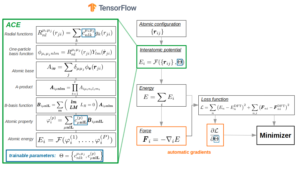
Specification of ACE potential

PACE potential specification consists of three parts:

1. Embeddings

i.e. how atomic energy \(E_i\) depends on ACE properties/densities \(\varphi\). Linear expansion \(E_i = \varphi\) is the trivial. Non-linear expansion, i.e. those, containing square root, gives more flexiblity and accuracy of final potential

Embeddings for ALL species (i.e. Al and Li):

• non-linear FinnisSinclairShiftedScaled

• 2 densities

• fs_parameters’: [1, 1, 1, 0.5]: $\(E_i = 1.0 * \varphi(1)^1 + 1.0 * \varphi(2)^{0.5} = \varphi^{(1)} + \sqrt{\varphi^{(2)}} \)$

job.input["potential"]["embeddings"]

2. Radial functions

Radial functions are orthogonal polynoms example:

• (a) Exponentially-scaled Chebyshev polynomials (λ = 5.25)

• (b) Power-law scaled Chebyshev polynomials (λ = 2.0)

• (c) Simplified spherical Bessel functions

Radial functions specification for ALL species pairs (i.e. Al-Al, Al-Li, Li-Al, Li-Li):

• based on the Simplified Bessel

• cutoff \(r_c=6.0\)

job.input["potential"]["bonds"]

3. B-basis functions

B-basis functions for ALL species type interactions, i.e. Al-Al, Al-Li, Li-Al, Li-Li blocks:

• maximum order = 4, i.e. body-order 5 (1 central atom + 4 neighbour densities)

• nradmax_by_orders: 15, 3, 2, 1

• lmax_by_orders: 0, 3, 2, 1

job.input["potential"]["functions"]

We will reduce the basis size for demonstartion purposes

job.input["potential"]["functions"]={'ALL': {'nradmax_by_orders': [15, 3, 2], 'lmax_by_orders': [0, 2, 1]}}

Fit/loss specification

Loss function specification

job.input["fit"]['loss']

Weighting

Energy-based weighting puts more “accent” onto the low energy-lying structures, close to convex hull

job.input["fit"]['weighting'] =  {
        ## weights for the structures energies/forces are associated according to the distance to E_min:
        ## convex hull ( energy: convex_hull) or minimal energy per atom (energy: cohesive)
        "type": "EnergyBasedWeightingPolicy",
        ## number of structures to randomly select from the initial dataset
        "nfit": 10000,         
        ## only the structures with energy up to E_min + DEup will be selected
        "DEup": 10.0,  ## eV, upper energy range (E_min + DElow, E_min + DEup)        
        ## only the structures with maximal force on atom  up to DFup will be selected
        "DFup": 50.0, ## eV/A
        ## lower energy range (E_min, E_min + DElow)
        "DElow": 1.0,  ## eV
        ## delta_E  shift for weights, see paper
        "DE": 1.0,
        ## delta_F  shift for weights, see paper
        "DF": 1.0,
        ## 0<wlow<1 or None: if provided, the renormalization weights of the structures on lower energy range (see DElow)
        "wlow": 0.95,        
        ##  "convex_hull" or "cohesive" : method to compute the E_min
        "energy": "convex_hull",        
        ## structures types: all (default), bulk or cluster
        "reftype": "all",        
        ## random number seed
        "seed": 42 
}

Minimization and backend specification

Type of optimizer: SciPy.minimize.BFGS. This optimizer is more efficient that typical optimizers for neural networks (i.e. ADAM, RMSprop, Adagrad, etc.), but it scales quadratically wrt. number of optimizable parameters. However number of trainable parameters for PACE potential is usually up to few thousands, so we gain a lot of accuracy during training with BFGS optimizer.

job.input["fit"]["optimizer"]

Maximum number of iterations by minimizer. Typical values are ~1000-1500, but we chose small value for demonstration purposes only

job.input["fit"]["maxiter"]=100

Batch size (number of simultaneously considered structures). This number should be reduced if there is not enough memory

job.input["backend"]["batch_size"]

For more details about these and other settings please refer to official documentation

Run fit

job.run()

pr.job_table()

Analyse fit

plot loss function

plt.plot(job["output/log/loss"])
plt.xlabel("# iter")
plt.ylabel("Loss")
plt.loglog()

plot energy per atom RMSE

plt.plot(job["output/log/rmse_epa"])
plt.xlabel("# iter")
plt.ylabel("RMSE E, eV/atom")
plt.loglog()

plot force component RMSE

plt.plot(job["output/log/rmse_f_comp"])
plt.xlabel("# iter")
plt.ylabel("RMSE F_i, eV/A")
plt.loglog()

load DataFrame with predictions

ref_df = job.training_data

pred_df = job.predicted_data

plt.scatter(pred_df["energy_per_atom_true"],pred_df["energy_per_atom"])

lims = [pred_df["energy_per_atom_true"].min(),pred_df["energy_per_atom_true"].max()]
plt.plot(lims, lims, ls="--",color="k")

plt.xlabel("DFT E, eV/atom")
plt.ylabel("ACE E, eV/atom")

plt.scatter(ref_df["forces"],pred_df["forces"])
lims = [pred_df["forces"].min(),pred_df["forces"].max()]
plt.plot(lims, lims, ls="--",color="k")

plt.xlabel("DFT F_i, eV/A")
plt.ylabel("ACE F_i, eV/A")

Check more in job.working_directory/report folder

! ls {job.working_directory}/report

How does an actual potential file look like ?

output_potential.yaml:

species:
    # Pure Al interaction block
  - speciesblock: Al
    radbase: SBessel
    radcoefficients: [[[1.995274603767268, -1.1940566258712266,...]]]
  
    nbody:
      # first order/ two-body functions = pair functions
      - {type: Al Al, nr: [1], nl: [0], c: [2.0970219095074687, -3.9539202281610351]}
      - {type: Al Al, nr: [2], nl: [0], c: [-1.8968648691718397, -2.3146574133175974]}
      - {type: Al Al, nr: [3], nl: [0], c: [1.3504952496800906, 1.5291190439028692]}
      - {type: Al Al, nr: [4], nl: [0], c: [0.040517989827027742, 0.11933504671036224]}
      ...
      # second order/ three-body functions 
      - {type: Al Al Al, nr: [1, 1], nl: [0, 0], c: [0.57788490809100468, -1.8642896163994958]}
      - {type: Al Al Al, nr: [1, 1], nl: [1, 1], c: [-1.0126646532267587, -1.2336078784112348]}
      - {type: Al Al Al, nr: [1, 1], nl: [2, 2], c: [-0.19324470046809467, 0.63954472122968498]}
      - {type: Al Al Al, nr: [1, 1], nl: [3, 3], c: [-0.22018334529075642, 0.32822679746839439]}
      ...
      # fifth order/ six-body functions 
      - {type: Al Al Al Al Al Al, nr: [1, 1, 1, 1, 1], nl: [0, 0, 0, 0, 0], lint: [0, 0, 0], c: [-0.71...]}
  
  
  # binary Al-Li interaction block    
  - speciesblock: Al Li      
     ...
     nbody:
      - {type: Al Li, nr: [1], nl: [0], c: [0.91843424537280882, -2.4170371138562308]}
      - {type: Al Li, nr: [2], nl: [0], c: [-0.88380210517336399, -0.97055273167339651]}
      ...
      - {type: Al Al Al Li Li, nr: [1, 1, 1, 1], nl: [1, 1, 0, 0], lint: [0, 0], c: [-0.0050,...]}
      ...
  # Pure Li interaction block      
  - speciesblock: Li
      nbody:
       ...
       - {type: Li Li Li, nr: [4, 4], nl: [3, 3], c: [-0.0059111333449957159, 0.035]}
       - {type: Li Li Li Li, nr: [1, 1, 1], nl: [0, 0, 0], lint: [0], c: [0.210,...]}
       ...
  # binary Al-Li interaction block    
  - speciesblock: Li Al
      nbody:
       ...
       - {type: Li Al Al, nr: [4, 4], nl: [3, 3], c: [0.014680736321211739, -0.030618474343919122]}
       - {type: Li Al Li, nr: [1, 1], nl: [0, 0], c: [-0.22827705573988896, 0.28367909613209036]}
       ...
  

output_potential.yaml is in B-basis form. For efficient LAMMPS implementaion it should be converted to so-called C-tilde form. This is already done by pyiron, but it could be also done manually by pace_yaml2yace utility. Check here for more details

Get LAMMPS potential and try some calculations

pace_lammps_potential = job.get_lammps_potential()
pace_lammps_potential

lammps_job = pr.create.job.Lammps("pace_lammps", delete_existing_job=True)

lammps_job.structure=pr.create.structure.bulk("Al", cubic=True)

lammps_job.potential=pace_lammps_potential

murn=pr.create.job.Murnaghan("LiAl_murn")

murn.ref_job = lammps_job

murn.run()

murn.plot()

Further reading

• Documentation

• pacemaker repository

• Bochkarev, A., Lysogorskiy, Y., Menon, S., Qamar, M., Mrovec, M. and Drautz, R. Efficient parametrization of the atomic cluster expansion. Physical Review Materials 6(1) 013804 (2022)

• Lysogorskiy, Y., Oord, C. v. d., Bochkarev, A., Menon, S., Rinaldi, M., Hammerschmidt, T., Mrovec, M., Thompson, A., Csányi, G., Ortner, C. and Drautz, R. Performant implementation of the atomic cluster expansion (PACE) and application to copper and silicon. npj Computational Materials 7(1), 1-12 (2021)

• Drautz, R. Atomic cluster expansion for accurate and transferable interatomic potentials. Physical Review B, 99(1), 014104 (2019)

Software used in this notebook

• pacemaker

• pyiron_atomistics

• LAMMPS

Validation workflows

For a complete set of validation workflows, see our previous workshop